Harnessing Octave: Your Free Alternative to Matlab for Science
Written on
Chapter 1: Introduction to Octave
GNU Octave is an open-source scientific programming language that provides a robust mathematical framework, a user-friendly syntax, and integrated visualization tools. This comprehensive suite is incredibly useful, featuring both a graphical user interface (GUI) and a command-line interface, resembling familiar Integrated Development Environments (IDEs) like those for Java or Python.
Octave is designed for tackling a wide array of mathematical challenges, developing simulations, and engaging in data science projects. If you have experience with Matlab or are searching for a quick prototyping tool for your scientific concepts, Octave is worth exploring. Let’s dive into practical examples to kickstart your journey with this software.
Section 1.1: Installation Procedures
To install Octave on Debian-based systems, such as Ubuntu, utilize the built-in package manager. Should you encounter missing packages, refer to the official command list for your specific operating system version. For Ubuntu 20.04, the installation command will look like this:
For Windows users, simply download the installer executable or unzip a provided file. The latest version available is 5.2, and you can find instructions for macOS and BSD systems in the relevant documentation.
Section 1.2: Understanding the GUI
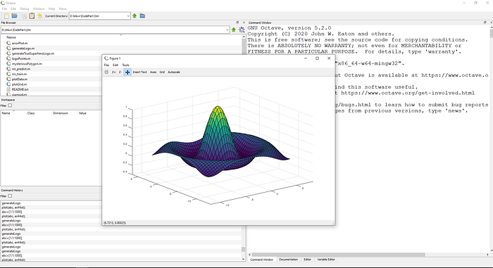
The Octave GUI is divided into four main sections. The largest area is the Command Window, where you can enter Octave commands interactively, with immediate results displayed.
At the bottom of the Command Window are three additional tabs:
- Documentation - An offline version of the Octave documentation, organized by topics like Data Types and Statements, which also includes a functions index with examples.
- Editor - A simple text editor for your Octave code with syntax completion features, though it maintains a minimalistic design.
- Variable Editor - Allows you to select and modify variable values, particularly useful for multidimensional variables.
On the left side, the window features three panels:
- File Browser - Lets you choose your project directory and manage files.
- Workspace - Displays all active variables along with brief descriptions (type, dimension, values, attributes).
- Commands History - Enables you to filter and search through previously executed commands.
Chapter 2: Working with Data
Data and variables are fundamental components of any programming project. Let’s explore how to define various types of variables and load files in Octave.
Section 2.1: Defining Variables
Defining variables in Octave is straightforward. You simply assign a name, use the "=" operator, and specify the desired value. This can include scalars such as integers, floating-point numbers, or strings (enclosed in quotes). If you input a value without a name, Octave assigns it to the variable "ans," which stores the last value entered in the command window.
To suppress output, you can end your command with a semicolon. Otherwise, the result will be printed to the console.
Section 2.2: Creating Vectors and Matrices
Vectors in Octave are defined by naming the vector and listing its values within square brackets. For a column vector, separate values with semicolons. Similarly, defining matrices involves separating row values with spaces and column values with semicolons.
For generating arrays filled with zeros or ones, you can use the functions zeros(m,n,k...) and ones(m,n,k...), where m, n, and k represent the dimensions.
To create a vector with discrete steps, specify the initial value, step size, and final value separated by colons.
Chapter 3: Data Access and Manipulation
One key aspect to remember is that Octave uses 1-based indexing, unlike many programming languages that start with 0. You specify indices in parentheses to access particular elements.
To load data, the load(filename.m) function is your best bet for files with comma-separated values. For example, if you have a file named "myData.m," you can load it into a variable as shown:
load('myData.m');
After loading, the size(variable) function can be used to check the dimensions of your data.
Chapter 4: Fundamental Linear Algebra in Octave
Octave's mathematical capabilities shine through in its built-in functions.
Section 4.1: Matrix Operations
For adding or subtracting matrices, use the "+" or "-" operators. When working with vectors, ensure compatibility in size.
To multiply matrices, remember the rule: the number of rows in the second matrix must equal the number of columns in the first. Use the "*" operator for multiplication. The output will be a new matrix.
For element-wise multiplication, use the dot operator before the multiplication sign (e.g., .*).
Section 4.2: Transposing and Solving Linear Systems
Transposing a matrix in Octave can be done with the "'" operator. To solve a system of linear equations, set up the matrices and use the left division operator "" for efficient computation.
Chapter 5: Visualization in Octave
To visualize data, Octave provides plotting functions. You can create 2D plots using the plot function, passing x and y coordinates along with style parameters.
For plotting functions, prepare a vector of x-coordinates and corresponding y-values, ensuring they are of equal length.
Section 5.1: Advanced Plotting Techniques
Octave also supports more complex visualizations. Explore functions like plot3, meshgrid, and surf for enhanced graphical representations.
A useful technique for filtering data involves using the find function to extract indices based on specified conditions, such as finding elements greater than a threshold.
Summary
This concise tutorial equips you with essential skills to navigate the Octave environment effectively. You now know how to define and load data, perform operations on vectors and matrices, and visualize your findings. Embrace Octave for your next prototyping project when you require a powerful yet simple tool that complements your existing programming setup.
